Chapter 3 Data transformation

The data we have are four csv files, which are grouped by four kinds of job titles: data science, data analyst, data engineer and business analyst. However, through scanning the dataset, we found that some of the tags inside the document are incorrect. Thus, the first step we take is through searching keywords inside the job title column and job description column, re-classifying our data. The sequence we labeled them is based on counts of their appearance inside the entire dataset. For instance, a job could both contain keywords for data science and data analyst. However, since data analyst appears more frequently, we tagged this job as data scientist. Meanwhile, we also fix typos and format similar meaning job titles into one, such as ‘Sr. Data scientist’ means the same as ‘Senior Data scientist’. Also, missing values are written in different formats such as “-1”, “not applicable” . They are replaced by NA. In addition, we separate the estimated salary into continuous data form: min_salary, max_salary and mean_salary to better analyze the dataset. Also, the location column is separated into “city” and “state” to be used inside the D3 interactive plot.

Here is a list of labels based on keyword search in data title and data description.

## [1] "is_ds_byjd" "is_da_byjt" "is_da_byjd" "is_ba_byjt"
## [5] "is_ba_byjd" "is_de_byjt" "is_de_byjd" "is_ds_byjt"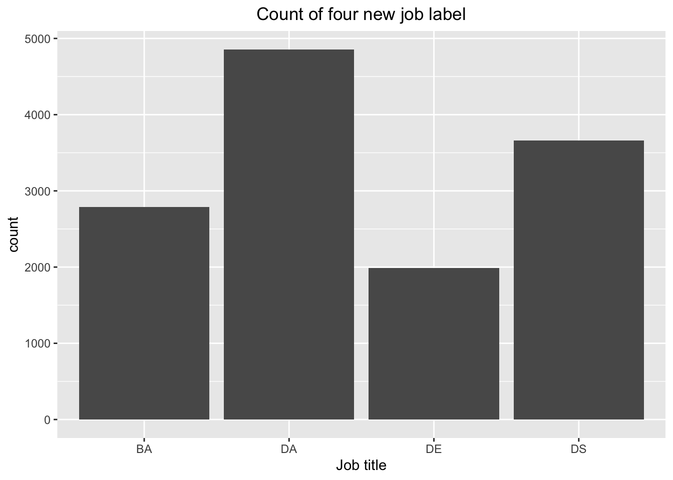

This graph indicates the counts of four types after we reclassify them. From the table, we could clearly see that DA>DS>BA>DE.